Dripread - Book

Mathematical Model

We will consider a mathematical model here which will help us to express our experimental observations in more general terms. You will find that the mathematical approach adopted and the result obtained is quite similar to what we encountered earlier with Radioactive Decay. So you will not have to plod your way through any new maths below, just a different application of the same form of mathematical analysis!

Let us start quite simply and assume that we vary only the thickness of the absorber. In other words we use an absorber of the same material (i.e. same atomic number) and the same density and use gamma-rays of the same energy for the experiment. Only the thickness of the absorber is changed.

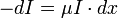
From our reasoning above it is easy to appreciate that the magnitude of ?I should be dependent on the radiation intensity as well as the thickness of the absorber, that is for an infinitesimally small change in absorber thickness:

$-d I \alpha I \cdot dx\,\!$

the minus sign indicating that the intensity is reduced by the absorber.

Turning the proportionality in this equation into an equality, we can write:

$-d I = \mu I \cdot dx\,\!$

where the constant of proportionality, ?, is called the Linear Attenuation Coefficient.

Dividing across by I we can rewrite this equation as:

$-\frac{d I}{I} = \mu \cdot dx$

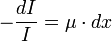
So this equation describes the situation for any tiny change in absorber thickness, dx. To find out what happens for the complete thickness of an absorber we simply add up what happens in each small thickness. In other words we integrate the above equation. Expressing this more formally we can say that for thicknesses from x = 0 to any other thickness x, the radiation intensity will decrease from I₀ to I_x, so that:

$- \int_{I_0}^{I_x} \frac{dI}{I} = \mu \int_{0}^x dx$

$\therefore \ln \left ( \frac{I_x}{I_0} \right ) = -\mu x$

$\therefore \frac{I_x}{I_0} = \text{exp}\ (-\mu x)$

$\therefore I_x = I_0\ \text{exp}\ (-\mu x)\,\!$

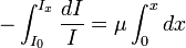
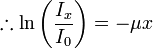
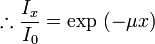
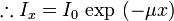
This final expression tells us that the radiation intensity will decrease in an exponential fashion with the thickness of the absorber with the rate of decrease being controlled by the Linear Attenuation Coefficient. The expression is shown in graphical form below. The graph plots the intensity against thickness, x. We can see that the intensity decreases from I₀, that is the number at x = 0, in a rapid fashion initially and then more slowly in the classic exponential manner.

Natural logarithm of intensity plotted against thickness.

Graphical representation of the dependence of radiation intensity on the thickness of absorber: Intensity versus thickness on the left and the natural logarithm of the intensity versus thickness on the right.

The influence of the Linear Attenuation Coefficient can be seen in the next figure. All three curves here are exponential in nature, only the Linear Attenuation Coefficient is different. Notice that when the Linear Attenuation Coefficient has a low value the curve decreases relatively slowly and when the Linear Attenuation Coefficient is large the curve decreases very quickly.

Exponential attenuation expressed using a small, medium and large value of the Linear Attenuation Coefficient, �.

The Linear Attenuation Coefficient is characteristic of individual absorbing materials. Some like carbon have a small value and are easily penetrated by gamma-rays. Other materials such as lead have a relatively large Linear Attenuation Coefficient and are relatively good absorbers of radiation:

Linear Attenuation Coefficients (in cm^-1) for a range of materials at gamma-ray energies of 100, 200 and 500 keV.
Absorber	100 keV	200 keV	500 keV
Air	0.000195	0.000159	0.000112
Water	0.167	0.136	0.097
Carbon	0.335	0.274	0.196
Aluminium	0.435	0.324	0.227
Iron	2.72	1.09	0.655
Copper	3.8	1.309	0.73
Lead	59.7	10.15	1.64

The materials listed in the table above are air, water and a range of elements from carbon (Z=6) through to lead (Z=82) and their Linear Attenuation Coefficients are given for three gamma-ray energies. The first point to note is that the Linear Attenuation Coefficient increases as the atomic number of the absorber increases. For example it increases from a very small value of 0.000195 cm^-1 for air at 100 keV to almost 60 cm^-1 for lead. The second point to note is that the Linear Attenuation Coefficient for all materials decreases with the energy of the gamma-rays. For example the value for copper decreases from about 3.8 cm^-1 at 100 keV to 0.73 cm^-1 at 500 keV. The third point to note is that the trends in the table are consistent with the analysis presented earlier.

Finally it is important to appreciate that our analysis above is only strictly true when we are dealing with narrow radiation beams. Other factors need to be taken into account when broad radiation beams are involved.

Basic Physics of Nuclear Medicine/Print version

Mathematical Model