by Wikibooks, open books for an open world
Available in 123 free installments
Owner:
For simple filters, a long wavelength approximation can be made to make the analysis of the system easier. When this assumption is valid (e.g. low frequencies) the components of the system behave as lumped acoustical elements. Equations relating the various properties are easily derived under these circumstances.
The following derivations assume long wavelength. Practical applications for most conditions are given later.
 Tpi for Low-Pass Filter

These are devices that attenuate the radiated sound power at higher frequencies. This means the power transmission coefficient is approximately 1 across the band pass at low frequencies(see figure to right).
This is equivalent to an expansion in a pipe, with the volume of gas located in the expansion having an acoustic compliance (see figure to right). Continuity of acoustic impedance (see Java Applet at: Acoustic Impedance Visualization) at the junction, see [1], gives a power transmission coefficient of:
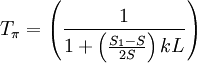
where k is the wavenumber (see [Wave Properties]), L & S1 are length and area of expansion respectively, and S is the area of the pipe.
The cut-off frequency is given by:
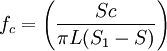
 Tpi for High-Pass Filter

These are devices that attenuate the radiated sound power at lower frequencies. Like before, this means the power transmission coefficient is approximately 1 across the band pass at high frequencies (see figure to right).
This is equivalent to a short side brach (see figure to right) with a radius and length much smaller than the wavelength (lumped element assumption). This side branch acts like an acoustic mass and applies a different acoustic impedance to the system than the low-pass filter. Again using continuity of acoustic impedance at the junction yields a power transmission coefficient of the form [1]:
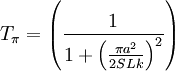
where a and L are the area and effective length of the small tube, and S is the area of the pipe.
The cut-off frequency is given by:
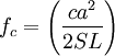
 Tpi for Band-Stop Filter

These are devices that attenuate the radiated sound power over a certain frequency range (see figure to right). Like before, the power transmission coefficient is approximately 1 in the band pass region.
Since the band-stop filter is essentially a cross between a low and high pass filter, one might expect to create one by using a combination of both techniques. This is true in that the combination of a lumped acoustic mass and compliance gives a band-stop filter. This can be realized as a helmholtz resonator (see figure to right). Again, since the impedance of the helmholtz resonator can be easily determined, continuity of acoustic impedance at the junction can give the power transmission coefficient as [1]:
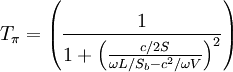
where Sb is the area of the neck, L is the effective length of the neck, V is the volume of the helmholtz resonator, and S is the area of the pipe. It is interesting to note that the power transmission coefficient is zero when the frequency is that of the resonance frequency of the helmholtz. This can be explained by the fact that at resonance the volume velocity in the neck is large with a phase such that all the incident wave is reflected back to the source [1].
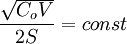
The zero power transmission coefficient location is given by:
This frequency value has powerful implications. If a system has the majority of noise at one frequency component, the system can be "tuned" using the above equation, with a helmholtz resonator, to perfectly attenuate any transmitted power (see examples below).
 Helmholtz Resonator as a Muffler, f = 60 Hz
|
 Helmholtz Resonator as a Muffler, f = fc
|
If the long wavelength assumption is valid, typically a combination of methods described above are used to design a filter. A specific design procedure is outlined for a helmholtz resonator, and other basic filters follow a similar procedure (see [1]).
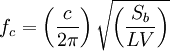
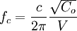
Two main metrics need to be identified when designing a helmholtz resonator [3]:
 where
where  .
. based on TL level. This constant is found from a TL graph (see HR pp. 6).
This will result in two equations with two unknowns which can be solved for the unknown dimensions of the helmholtz resonator. It is important to note that flow velocities degrade the amount of transmission loss at resonance and tend to move the resonance location upwards [3].
In many situations, the long wavelength approximation is not valid and alternative methods must be examined. These are much more mathematically rigorous and require a complete understanding acoustics involved. Although the mathematics involved are not shown, common filters used are given in the section that follows.
