by Wikibooks, open books for an open world
Available in 123 free installments
Owner:
The performance of the loudspeaker is first measured by its velocity response, which can be found directly from the equivalent circuit of the system. As the goal of most loudspeaker designs is to improve the bass response (leaving high-frequency production to a tweeter), low frequency approximations will be made as much as possible to simplify the analysis. First, the inductance of the voice coil, LE, can be ignored as long as  . In a typical loudspeaker, LE is of the order of 1 mH, while RE is typically 8?, thus an upper frequency limit is approximately 1 kHz for this approximation, which is certainly high enough for the frequency range of interest.
Another approximation involves the radiation impedance, ZRAD. It can be shown [1] that this value is given by the following equation (in acoustical ohms):
![Z_{RAD} = \frac{\rho_0c}{\pi a^2}\left[\left(1 - \frac{J_1(2ka)}{ka}\right) + j\frac{H_1(2ka)}{ka}\right]](4b21bbd711bf09435ad4547bc290fdc3.png)
Where J1(x) and H1(x) are types of Bessel functions. For small values of ka,
 |
and |  |
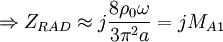 |
Hence, the low-frequency impedance on the loudspeaker is represented with an acoustic mass MA1 [1]. For a simple analysis, RE, MMD, CMS, and RMS (the transducer parameters, or Thiele-Small parameters) are converted to their acoustical equivalents. All conversions for all parameters are given in Appendix A. Then, the series masses, MAD, MA1, and MAB, are lumped together to create MAC. This new circuit is shown below.

Figure 4. Low-Frequency Equivalent Acoustic Circuit
Unlike sealed enclosure analysis, there are multiple sources of volume velocity that radiate to the outside environment. Hence, the diaphragm volume velocity, UD, is not analyzed but rather U0 = UD + UP + UL. This essentially draws a ?bubble? around the enclosure and treats the system as a source with volume velocity U0. This ?lumped? approach will only be valid for low frequencies, but previous approximations have already limited the analysis to such frequencies anyway. It can be seen from the circuit that the volume velocity flowing into the enclosure, UB = ? U0, compresses the air inside the enclosure. Thus, the circuit model of Figure 3 is valid and the relationship relating input voltage, VIN to U0 may be computed.
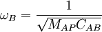
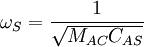
In order to make the equations easier to understand, several parameters are combined to form other parameter names. First, ?B and ?S, the enclosure and loudspeaker resonance frequencies, respectively, are:
 |
 |
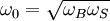
Based on the nature of the derivation, it is convenient to define the parameters ?0 and h, the Helmholtz tuning ratio:
 |
 |
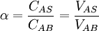
A parameter known as the compliance ratio or volume ratio, ?, is given by:
Other parameters are combined to form what are known as quality factors:
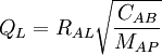 |
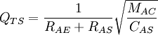 |
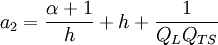
This notation allows for a simpler expression for the resulting transfer function [1]:

where
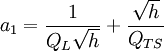 |
 |
 |
