Acoustics

by Wikibooks, open books for an open world

Available in 123 free installments

Owner:

Chebyshev Alignment

The Chebyshev algorithm is an alternative to the Butterworth algorithm. For the Chebyshev response, the maximally-flat passband restriction is abandoned. Now, a ripple, or fluctuation is allowed in the pass band. This allows a steeper transition or roll-off to occur. In this type of application, the low-frequency response of the loudspeaker can be extended beyond what can be achieved by Butterworth-type filters. An example plot of a Chebyshev high-pass response with 0.5 dB of ripple against a Butterworth high-pass response for the same $? 3 d B$ is shown below.

Figure 6: Chebyshev vs. Butterworth High-Pass Response.

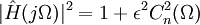
The Chebyshev response is defined by [4]:

$|\hat{H}(j\Omega)|^2 = 1 + \epsilon^2C^2_n(\Omega)$

$C n (?)$ is called the Chebyshev polynomial and is defined by [4]:

$C_n(\Omega) = \big\lbrace$	$cos[n cos ? 1 (?)]$	$\| ? \| < 1$
$C_n(\Omega) = \big\lbrace$	$cosh[n cosh ? 1 (?)]$	$\| ? \| > 1$

Fortunately, Chebyshev polynomials satisfy a simple recursion formula [4]:

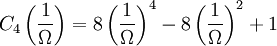
C 0 (x) = 1

C 1 (x) = x

C n (x) = 2 x C n ? 1 ? C n ? 2

For more information on Chebyshev polynomials, see the Wolfram Mathworld: Chebyshev Polynomials page.

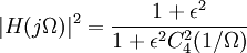
When applying the high-pass transformation to the 4th order form of $|\hat{H}(j\Omega)|^2$ , the desired response has the form [1]:

$|H(j\Omega)|^2 = \frac{1+\epsilon^2}{1+\epsilon^2C^2_4(1/\Omega)}$

The parameter $?$ determines the ripple. In particular, the magnitude of the ripple is $10log[1 + ? 2]$ dB and can be chosen by the designer, similar to B in the quasi-Butterworth case. Using the recursion formula for $C n (x)$ ,

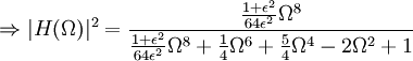
$C_4\left(\frac{1}{\Omega}\right) = 8\left(\frac{1}{\Omega}\right)^4 - 8\left(\frac{1}{\Omega}\right)^2 + 1$

Applying this equation to $| H (j ?) | 2$ [1],

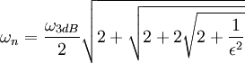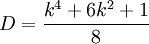
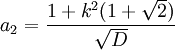
$\Rightarrow \|H(\Omega)\|^2 = \frac{\frac{1 + \epsilon^2}{64\epsilon^2}\Omega^8}{\frac{1 + \epsilon^2}{64\epsilon^2}\Omega^8 + \frac{1}{4}\Omega^6 + \frac{5}{4}\Omega^4 - 2\Omega^2 + 1}$
$\Omega = \frac{\omega}{\omega_n}$	$\omega_n = \frac{\omega_{3dB}}{2}\sqrt{2 + \sqrt{2 + 2\sqrt{2+\frac{1}{\epsilon^2}}}}$

Thus, the design equations become [1]:

$\omega_0 = \omega_n\sqrt[8]{\frac{64\epsilon^2}{1+\epsilon^2}}$	$k = \rm{tanh}\left[\frac{1}{4}\rm{sinh}^{-1}\left(\frac{1}{\epsilon}\right)\right]$	$D = \frac{k^4 + 6k^2 + 1}{8}$
$a_1 = \frac{k\sqrt{4 + 2\sqrt{2}}}{\sqrt[4]{D}},$	$a_2 = \frac{1 + k^2(1+\sqrt{2})}{\sqrt{D}}$	$a_3 = \frac{a_1}{\sqrt{D}}\left[1 - \frac{1 - k^2}{2\sqrt{2}}\right]$