Acoustics

by Wikibooks, open books for an open world

Available in 123 free installments

Owner:

Quasi-Butterworth Alignment

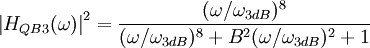
The quasi-Butterworth alignments do not have as well-defined of an algorithm when compared to the Butterworth alignment. The name ?quasi-Butterworth? comes from the fact that the transfer functions for these responses appear similar to the Butterworth ones, with (in general) the addition of terms in the denominator. This will be illustrated below. While there are many types of quasi-Butterworth alignments, the simplest and most popular is the 3rd order alignment (QB3). The comparison of the QB3 magnitude-squared response against the 4th order Butterworth is shown below.

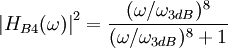$\left|H_{QB3}(\omega)\right|^2 = \frac{(\omega/\omega_{3dB})^8}{(\omega/\omega_{3dB})^8 + B^2(\omega/\omega_{3dB})^2 + 1}$

$\left|H_{B4}(\omega)\right|^2 = \frac{(\omega/\omega_{3dB})^8}{(\omega/\omega_{3dB})^8 + 1}$

Notice that the case $B = 0$ is the Butterworth alignment. The reason that this QB alignment is called 3rd order is due to the fact that as B increases, the slope approaches 3 dec/dec instead of 4 dec/dec, as in 4th order Butterworth. This phenomenon can be seen in Figure 5.

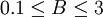
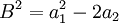
Figure 5: 3rd-Order Quasi-Butterworth Response for $0.1 \leq B \leq 3$

Equating the system response $| H (s) | 2$ with $| H Q B 3 (s) | 2$ , the equations guiding the design can be found [1]:

$a_3 = \sqrt{2a_2}$

$a_2 > 2 + \sqrt{2}$